PostgreSQL Internals - Module 5: Query pipeline

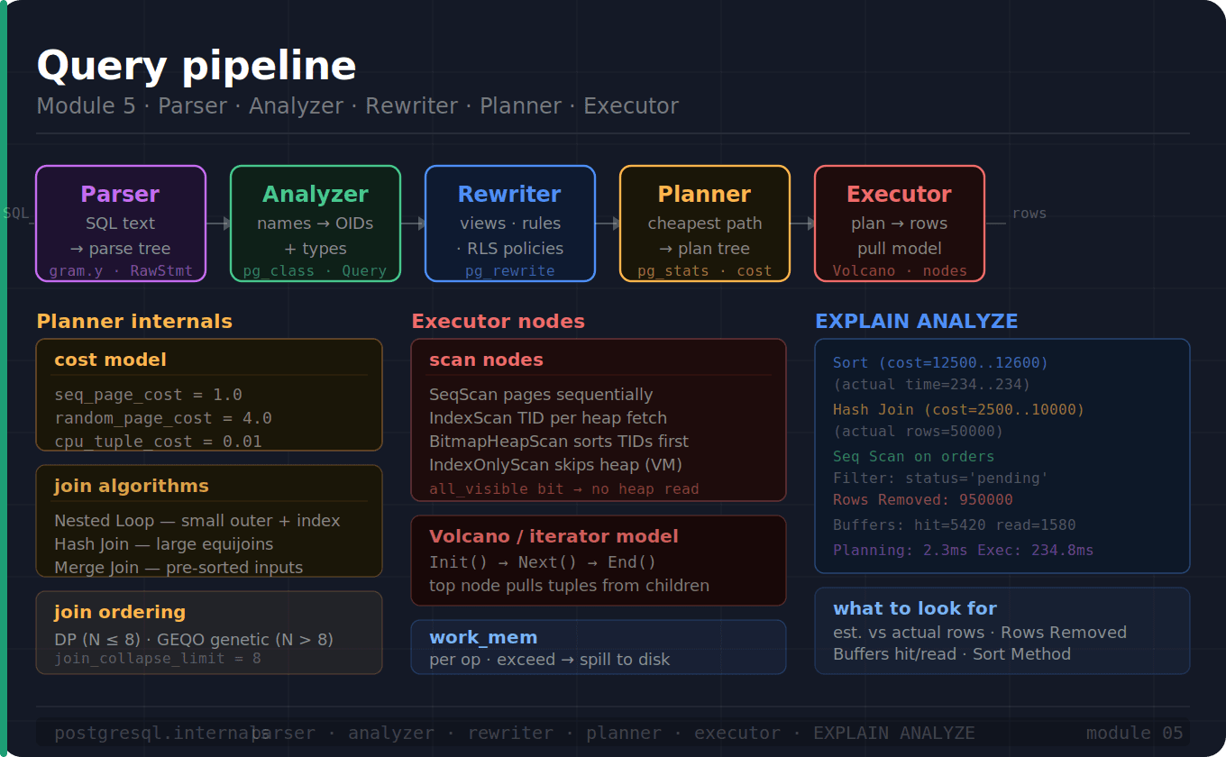
In the previous blog, we have explored about the WAL and how it will helpful for Checkpoints, Crash Recovery and Replications.

Every SQL statement you send to PostgreSQL travels through a precise pipeline before a single row is returned. This post traces that journey end-to-end, from raw text bytes arriving over the wire to result rows going back to the client.

Part 1: The Big Picture

Consider a client sending the query: SELECT * FROM orders WHERE status = 'pending' ORDER BY created_at. Here's how it travels through the pipeline:

"SELECT * FROM orders WHERE status = 'pending' ORDER BY created_at"

SQL Statement → Parser (returns Parse Tree) → Analyzer (returns Query Tree) → Rewriter applies Rules, Views (returns a list of Query Tree) → Planner (return Plan Tree) → Executor → Result Rows

In the above flow, the output of the previous stage will act as input to the next stage.

Part 2: The Parser

Input: Raw SQL statement

Output: a RawStmt parse tree

Checks: Checks for syntax purely, no semantic meaning

This parser lives in src/backend/parser/gram.y - a yacc/bison grammar file. It performs only "syntactic validation" i.e., it checks that the SQL is grammatically correct but has no idea whether the tables or columns actually exist. It uses a LALR(1) parsing algorithm, tokens are read left-to-right, with decisions made using a single token of lookahead.

What the parser produces

Input:

SELECT id, name FROM orders o WHERE o.status = 'pending';

Parser Pipeline

SQL text: "SELECT id,name FROM orders o WHERE o.status = 'pending'"
│
V
Lexer (scan.l)
│  tokenizes into:
│  SELECT  id,name  FROM  orders  WHERE  status  =  $1
│  (keyword)(ident)(sep)(ident)(keyword)(ident)(keyword)(ident)(op)(param)
│
V
Parser (gram.y)
│  builds parse nodes:
│  SelectStmt
│    targetList: [ResTarget(ColumnRef("id"))]
│    targetList: [ResTarget(ColumnRef("name"))]
│    fromClause: [RangeVar("orders")]
│    whereClause: A_Expr("=", ColumnRef("status"), ParamRef(1))
│
V
RawStmt (List of raw parse nodes)

Output: Parse Tree of C structs

SelectStmt
|
|--- targetList
|     |- ResTarget → ColumnRef("id")
|     |- ResTarget → ColumnRef("name")
|--- fromClause
|     |- RangeVar (relname="orders", inh=true)
|--- whereClause
|     |- A_Expr (op="=")
|          |- ColumnRef("status")
|          |- A_Const(str="pending")

At this point "orders" is just a string, not a table. "status" is just a name, not a column. The parser doesn't know or care.

Parse Node Types - the Full Taxonomy

/* Statement nodes */
SelectStmt, InsertStmt, UpdateStmt, DeleteStmt
CreateStmt, AlterTableStmt, DropStmt
TransactionStmt, ExplainStmt, CopyStmt
VacuumStmt, AnalyzeStmt, IndexStmt

/* Expression nodes */
A_Expr        — binary/unary operator expression
ColumnRef     — reference to a column (just a name at this stage)
A_Const       — a literal constant (integer, float, string, bool, null)
ParamRef      — a query parameter ($1, $2, ...)
FuncCall      — function call (name + args, no OID yet)
TypeCast      — explicit cast: expr::type
SubLink       — subquery in expression context (IN, EXISTS, ANY, ALL)
CaseExpr      — CASE WHEN ... THEN ... ELSE ... END
CoalesceExpr  — COALESCE(...)
BoolExpr      — AND, OR, NOT
A_ArrayExpr   — ARRAY[...]
RowExpr       — ROW(...)

What the parser catches

-- Syntax error caught by parser
SELECT * FORM orders; -- ERROR: syntax error at "FORM"
SELECT * FROM;        -- ERROR: syntax error at ";"

-- Not caught by parser (semantic errors)
SELECT * FROM nonexistent_table; -- passes the parser phase
SELECT fake_col FROM orders;     -- passes the parser phase

Part 3: The Analyzer (Semantic Analysis)

Input: RawStmt parse tree

Output: Query tree (fully resolved, typed)

The analyzer lives in src/backend/parser/analyze.c. This is where PostgreSQL looks up system catalogs like pg_class, pg_attribute, pg_type, pg_operator, and others - to resolve every name to an OID (Object Identifier) and every expression to a type.

What the analyzer does

Note: The walkthrough below follows directly from the parse tree produced in Part 2, and the same resolution process applies to more complex queries.

RangeVar("orders")

1. Lookup pg_class for the relname = 'orders'

2. Resolves to OID 24601 (example value) and relkind = 'r' (regular table)

3. Replace with RangeTblEntry struct like below:

rtable[1]: RTE_RELATION relid=24601 (orders) alias="o"

ColumnRef("id")

1. Lookup pg_attribute WHERE attrelid=24601(orders) AND attname='status'

2. Resolve to atttypid=22 (integer type OID), attnum=1 (position of this column in table)

3. Replace with Var struct like below

o.id → Var(varno=1, varattno=1, vartype=INT4OID)
o.name → Var(varno=1, varattno=2, vartype=TEXTOID)
o.status → Var(varno=1, varattno=3, vartype=TEXTOID)

A_Const(str="pending")

1. type = text which will be inferred from the context

2. Replace with Const struct like below:

Const(consttype=25, constvalue="pending")

A_Expr(op="=", left=ColumnRef, right=A_Const)

1. Lookup pg_operator WHERE oprname = '=' AND oprleft = 25 AND oprright = 25

2. Resolve to operator OID 98 (for =).

3. Replaces with OpExpr struct like below:

OpExpr(opno=98, args=[
     Var(varno=1, varattno=3, vartype=TEXTOID), 
     Const(consttype=25, constvalue="pending")
  ]
)

After analysis, every node in the tree is fully typed and resolved to their identifiers (OIDs). Unknown tables or columns fails here with the errors we used to seeing:

SELECT * FROM nonexistent_table;
-- ERROR:  relation "nonexistent_table" does not exist

SELECT fake_col FROM orders;
-- ERROR:  column "fake_col" does not exist

The Query Struct

typedef struct Query {
    CmdType      commandType;    /* SELECT, INSERT, UPDATE, DELETE */
    bool         hasAggs;        /* has aggregate functions? */
    bool         hasSubLinks;    /* has subqueries? */
    bool         hasWindowFuncs; /* has window functions? */
    List        *rtable;         /* range table: list of all tables used */
    FromExpr    *jointree;       /* FROM and WHERE clauses */
    List        *targetList;     /* SELECT columns / SET clauses */
    Node        *havingQual;     /* HAVING clause */
    List        *groupClause;    /* GROUP BY */
    List        *sortClause;     /* ORDER BY */
    Node        *limitOffset;    /* OFFSET */
    Node        *limitCount;     /* LIMIT */
} Query;

Part 4: The Rewriter

Input: Query tree

Output: List of Query trees (may expand one query into multiple)

The rewriter lives in src/backend/rewrite/rewriteHandler.c and applies rewrite rules stored in pg_rewrite. One such important use case being view expansion.

View expansion

CREATE VIEW active_orders AS
  SELECT * FROM orders WHERE status != 'cancelled';

-- Now suppose we ran the following query
SELECT id FROM active_orders WHERE created_at > '2026-04-21';

The rewriter:

1. Detects active_orders is a view (from pg_class.relkind = 'v' )

2. Fetches the view definition from pg_rewrite .

3. Substitutes the view's SELECT in place of the RangeTblEntry

4. Merges WHERE created_at > '2026-04-21' with the view's quals.

Result after rewriting:

-- After rewriting
SELECT id FROM orders
WHERE status != 'cancelled' AND created_at > '2026-04-21';

The planner never sees the view name, it sees the fully expanded query and it's query tree. Views have zero runtime overhead - they are purely a rewrite-time substitution.

Row Security Policies

CREATE POLICY user_isolation ON orders
  USING (user_id = current_user_id());

The rewriter appends the policy's USING expression to the WHERE clause of every query touching that table. The planner receives a query that already has the security filter added.

Part 5: The Planner

Input: Query tree

Output: PlannedStmt containing a tree of Plan nodes

The planner is the most intellectually complex part of PostgreSQL (src/backend/optimizer/). Its job: enumerate every possible execution strategy and pick the cheapest one.

It's organized into three main phases:

1. Preprocessing: Simplify quals, pull up subqueries, reduce ops

2. Path Generation: Enumerate all access paths for each relation and join

3. Plan Building: Convert the cheapest path tree into a Plan tree

Step 1: Preprocessing

SELECT * FROM orders
WHERE status = 'pending'
   AND (1 = 1)                    -- constant true --> removed
   AND amount > 0 AND amount > 50 -- simplified to amount > 50
   AND id IN (SELECT order_id FROM order_items WHERE qty > 10);

The preprocessor:

• Folds constants: 1=1 which will true always and it won't effect the results anyway, so will be removed from quals.

• Simplifies redundant predicates: amount > 0 and amount > 50 simply means amount > 50.

• Attempts to pull up the subquery as a join (if safe to do so)

• Flattens nested AND/OR into flat clause lists.

Step 2: Generate RelOptInfo for each relation

For every table in the query, the planner creates a RelOptInfo struct and gathers statistics from pg_statistic (populated by ANALYZE):

-- What ANALYZE collects, readable via pg_stats:
SELECT attname,
       n_distinct,          -- estimated distinct values
       correlation,         -- physical sort order correlation
       most_common_vals,    -- MCV list
       most_common_freqs,   -- frequency of each MCV
       histogram_bounds     -- bucket boundaries for non-MCV values
FROM pg_stats
WHERE tablename = 'orders' AND attname = 'status';

Step 3: Estimate selectivity and row counts

For each WHERE predicate, the planner estimates its selectivity i.e. what fraction of rows expected to pass the filter:

WHERE status = 'pending'
-- Look up 'pending' in most_common_vals → freq = 0.15
-- Estimated rows = 1,000,000 * 0.15 = 150,000

WHERE created_at > '2026-01-01'
-- Use histogram_bounds to find fraction above threshold
-- Estimated rows = 1,000,000 * 0.35 = 350,000

WHERE status = 'pending' AND created_at > '2026-01-01'
-- Assume independence (unless extended stats created):
-- 1,000,000 * 0.15 * 0.35 = 52,500 rows

Step 4: Generate access paths for each relation

For a single table orders, the planner generates all the possible paths to access that table by various modes of scanning like seqscan (read page by page sequentially), index scan (scan the index) etc. To decide what best among these, planner estimates the cost of each possible path/scan and picks the best one.

SeqScan(orders)
  cost = seq_page_cost × pages + cpu_tuple_cost × rows
       = 1.0 × 10000 + 0.01 × 1000000
       = 20,000

IndexScan(orders_status_idx)
  cost = random_page_cost × index_pages + cpu_index_tuple_cost × index_rows
       + random_page_cost × heap_pages_fetched
       = 4.0 × 500 + 0.005 × 150000 + 4.0 × 15000
       = 2000 + 750 + 60000 = 62,750  ← more expensive than seqscan here!

BitmapIndexScan + BitmapHeapScan
  cost = index_cost + 0.1 × heap_pages (sequential after sort)
       = 750 + 0.1 × 15000 = 2,250   ← much cheaper

This is why a low-selectivity index is often skipped - the planner does real cost math, not guesswork.

The cost parameters

SHOW seq_page_cost; -- 1.0   (baseline: cost of one sequential page read)
SHOW random_page_cost;  -- 4.0   (default: random I/O is 4× slower)
                        -- set to 1.1 for SSDs!
SHOW cpu_tuple_cost; -- 0.01
SHOW cpu_index_tuple_cost; -- 0.005
SHOW cpu_operator_cost; -- 0.0025
SHOW effective_cache_size; -- 4GB (planner's estimate of OS + PG cache)

Step 5: Join ordering generation

For multi-table queries, the planner must find the optimal join order. With N tables there are N! possible orderings. For small N (<= join_collapse_limt (default 8)), the planner uses dynamic programming to find the true optimum. For large N, it switches to a Genetic Algorithm (GEQO)

-- Three-table join: orders, customers, products
-- Possible orderings: 3! = 6
-- (orders ⋈ customers) ⋈ products
-- (orders ⋈ products) ⋈ customers
-- (customers ⋈ products) ⋈ orders
-- (customers ⋈ orders) ⋈ products
-- (products ⋈ customers) ⋈ orders
-- (products ⋈ orders) ⋈ customers

The Planner tries all possible 6 combinations, estimates the cost of each and picks the cheapest in all of them.

Step 6: Choose Join Algorithms

For each join, planner has three algorithms, from which it picks the best possible one. The three algorithms are:

1. Nested Loop Join

2. Hash Join

3. Merge Join

Nested Loop Join

Sample Algorithm
for each outer row:
    scan inner for matching rows

• Cost would be = outer_rows x inner_scan_cost

• Good for small outer table and indexed inner table.

Hash Join

Sample Algorithm
build has table from smaller relation
probe with larger relation

• Cost would be = build_cost (for hash) + probe_cost

• Good for large equijoins, no useful indexes

Merge Join

Sample Algorithm
sort both inputs on join key and merge them

• Cost would be = sort_cost_outer_table + sort_cost_inner_table + merge_cost

• Good for inputs that are already sorted (index scan) or ORDER BY on join key

Step 7: Build the final plan tree

Once the cheapest path is choosen, at this phase it generates the PlannedStmt containing the tree of PlannedStmt nodes which will be passed to the Executor phase. Here I am showing that plan using EXPLAIN.

EXPLAIN SELECT o.id, c.name
FROM orders o JOIN customers c ON o.customer_id = c.id
WHERE o.status = 'pending'
ORDER BY o.created_at;
---------------------------------------------------------------
EXPLAIN PLAN generated on cheapest final plan tree
---------------------------------------------------------------
Sort  (cost=12500..12600 rows=50000)
  Sort Key: o.created_at
  →  Hash Join  (cost=2500..10000 rows=50000)
        Hash Cond: (o.customer_id = c.id)
        →  Seq Scan on orders o  (cost=0..8000 rows=50000)
              Filter: (status = 'pending')
        →  Hash  (cost=1500..1500 rows=100000)
              →  Seq Scan on customers c  (cost=0..1500 rows=100000)

Part 6: The Executor

Input: PlannedStmt

Output: Tuple stream (rows returned to client)

The executor uses the Volcano/Iterator model, where every plan node implements three operations:

ExecInitNode(node) /* open: allocate state, initialize children */
ExecProcNode(node) /* next: return one tuple at a time (or NULL if done) */
ExecEndNode(node)  /* close: free resources */

The top node is called with ExecProcNode(). It calls its children, which call their children, pulling tuples up through the tree one at a time. This is the pull model i.e., the data flows upward on demand.

A plan tree is a collection of nodes each with their own responsibilities. One node's responsibility is to read the data from the page, while other is to order the data fetched by other node etc. Let's see some of those such nodes.

Scan nodes (leaves of the plan tree)

Like

1. SeqScan

2. IndexScan

3. BitmapIndexScan

4. IndexOnlyScan

SeqScan
  reads pages from the buffer pool sequentially
  applies filter quals to each tuple
  calls heap_getnext() in a loop

IndexScan
  calls index_getnext() to get TIDs from index
  for each TID: calls heap_fetch() to get the tuple
  applies any remaining filter quals

BitmapIndexScan + BitmapHeapScan
  BitmapIndexScan: scans index, builds a bitmap of matching page+offset
  BitmapHeapScan:  reads pages in physical order using the bitmap
                   (avoids random I/O by sorting TIDs first)

IndexOnlyScan
  calls index_getnext()
  checks visibility map — if all_visible: return tuple from index leaf
  if NOT all_visible: fetch from heap to check visibility
  never reads heap at all for fully-visible pages

Join Nodes

Like

1. NestLoop

2. HashJoin

3. MergeJoin

NestLoop
  outer_slot = ExecProcNode(outer_child)
  while outer_slot not NULL:
    inner_slot = ExecProcNode(inner_child)  ← rescanned for each outer
    while inner_slot not NULL:
      if qual matches: emit joined tuple
      inner_slot = ExecProcNode(inner_child)
    outer_slot = ExecProcNode(outer_child)

HashJoin
  ExecInitNode: build hash table from inner child
  ExecProcNode:
    outer_slot = ExecProcNode(outer_child)
    hash outer_slot on join key
    probe hash table → emit matching tuples

MergeJoin
  assumes both inputs sorted on join key
  merge using two pointers advancing through sorted streams

Other nodes

Sort         reads all tuples from child, sorts in work_mem
             if > work_mem: spills to temp files (external merge sort)

HashAgg      GROUP BY using a hash table (one entry per group)
             if > work_mem: spills to disk

Limit        counts tuples, stops after N
Append       union of multiple children (used for partitioned tables)
Result       evaluates a constant expression (no child scan)
Materialize  buffers child output (lets inner of NestLoop re-read)

Part 7: EXPLAIN ANALYZE

EXPLAIN (ANALYZE, BUFFERS, FORMAT TEXT)
SELECT o.id, c.name
FROM orders o
JOIN customers c ON o.customer_id = c.id
WHERE o.status = 'pending'
ORDER BY o.created_at
LIMIT 100;

Sample output:

Limit  (cost=14234..14234 rows=100 width=36)
       (actual time=234.5..234.6 rows=100 loops=1)
  ->  Sort  (cost=14234..14359 rows=50000 width=36)
            (actual time=234.5..234.5 rows=100 loops=1)
        Sort Key: o.created_at
        Sort Method: top-N heapsort  Memory: 36kB     ← LIMIT lets planner use heapsort
        ->  Hash Join  (cost=2500..10000 rows=50000 width=36)
                       (actual time=45.2..198.3 rows=50000 loops=1)
              Hash Cond: (o.customer_id = c.id)
              Buffers: shared hit=8420 read=1580       ← 8420 from cache, 1580 from disk
              ->  Seq Scan on orders o
                           (cost=0..8000 rows=50000 width=28)
                           (actual time=0.1..120.4 rows=50000 loops=1)
                    Filter: (status = 'pending')
                    Rows Removed by Filter: 950000     ← 950k rows scanned but discarded
                    Buffers: shared hit=5420 read=1580
              ->  Hash  (cost=1500..1500 rows=100000 width=16)
                         (actual time=44.8..44.8 rows=100000 loops=1)
                    Buckets: 131072  Batches: 1  Memory Usage: 5452kB
                    ->  Seq Scan on customers c
                                 (cost=0..1500 rows=100000 width=16)
                                 (actual time=0.1..22.1 rows=100000 loops=1)
                                 Buffers: shared hit=3000
Planning Time: 2.3 ms
Execution Time: 234.8 ms

How to read

Every node shows estimated (cost=X..Y rows=N) and actual (actual time=A..B rows=N loops=L)

• cost=0..1500

  • 0 - cost to return fist row/tuple

  • 1500 - cost to return all the tuples

• actual time=0.1..22.1

  • 0.1 - time taken for first row to return (ms)

  • 22.1 - total time taken for all rows to return

• rows=50000

  • actual rows returned

• loops=1

  • how many times this node was executed.

• Buffers: shared hit=5420 read=1580

  • hit = pages served from shared_buffers (no disk I/O)

  • read = pages read from disk

  • From we can calculate cache hit ratio = (5420 / (5420 + 1580))x100% = 77% of data read from the cache itself

Key things to look for

Consider you have table with 1M rows

Rows Removed by Filter: 950000
→ index would help here — you're scanning 1M rows to get 50K

Sort Method: external merge  Disk: 128000kB
→ increase work_mem

Hash Batches: 8  (instead of 1)
→ hash table spilled to disk — increase work_mem

actual rows >> estimated rows
→ stale statistics — run ANALYZE

loops=50000 on an inner node
→ nested loop with 50K outer rows — consider hash join
   set enable_nestloop = off to test

Part 8: Advanced Executions

Parallel Query

Since PostgreSQL 9.6, the executor can parallelize sequential scans and joins.

SET max_parallel_workers_per_gather = 4;

-- Execute
EXPLAIN SELECT count(*) FROM large_orders WHERE amount > 100;

Output:

Finalize Aggregate  (cost=284000..284001 rows=1)
  → Gather  (cost=283999..284000 rows=1 workers=4)
        → Partial Aggregate
              → Parallel Seq Scan on large_orders
                    Filter: (amount > 100)

How it works:

Leader process
  │
  │── fork → Worker 1 ── scans blocks 0..249999
  │── fork → Worker 2 ── scans blocks 250000..499999
  │── fork → Worker 3 ── scans blocks 500000..749999
  │── fork → Worker 4 ── scans blocks 750000..999999
  │
  │  Each worker computes Partial Aggregate (partial count)
  │  Sends result through a DSM (dynamic shared memory) queue
  │
  Gather node collects partial results
  Finalize Aggregate combines partial counts → final count

Block assignment uses a parallel block scan, workers atomically increment a shared block counter, so each block is scanned by exactly one worker.

Query Caching - The Plan Cache

PostgreSQL caches plans for prepared statements:

PREPARE get_orders(text) AS
    SELECT * FROM orders WHERE status = $1 ORDER BY created_at;

EXECUTE get_orders('pending');
EXECUTE get_orders('cancelled');

Generic vs Custom Plans

For the first 5 executions, PostgreSQL builds a custom plan - it substitues the actual parameter value and plans with full statistics knowledge.

After 5 executions, it compares the average custom plan cost versus a generic plan (one built without knowing the parameter value). If the generic plan is cheaper (e.g., always a seq scan regardless of parameter), PostgreSQL switches to the generic plan.

-- See what plan is being used:
EXPLAIN (ANALYZE) EXECUTE get_orders('pending');
-- Look for "Generic Plan" or "Custom Plan" in output (PG 16+)

-- Force generic plan:
SET plan_cache_mode = force_generic_plan;

-- Force custom plan (re-plan every execution):
SET plan_cache_mode = force_custom_plan;

This matters for skewed data — if status='pending' has 80% of rows but status='archived' has 0.001%, a generic plan can be catastrophically wrong for one of them.

Conclusion

Every query you write travels farther than it looks. A single SELECT passes through a lexer, a grammar parser, a semantic analyzer resolving names to OIDs, a rewriter substituting views and policies, a cost-based planner enumerating thousands of execution strategies, and finally an executor pulling tuples through a tree of nodes — one row at a time.

Understanding this pipeline changes how you think about performance. Slow query? Now you know whether to look at statistics staleness (Analyzer/Planner), missing indexes (Path Generation), skewed plan caching (Generic vs Custom), or work_mem pressure (Sort/HashAgg). EXPLAIN ANALYZE stops being a black box and becomes a direct window into the decisions PostgreSQL made at each stage.

In the next module, we'll go deeper into Indexing Internals.

What's Next → Module 6: Indexing Internals

In Module 6, we'll go deep into how PostgreSQL builds and traverses B-Tree indexes, how the page layout looks on disk, what happens during index splits, and why an index scan can sometimes hurt more than it helps. We'll also cover GIN, GiST, and BRIN — when each one exists and what problem it was designed to solve.