The Anatomy of Query Structure

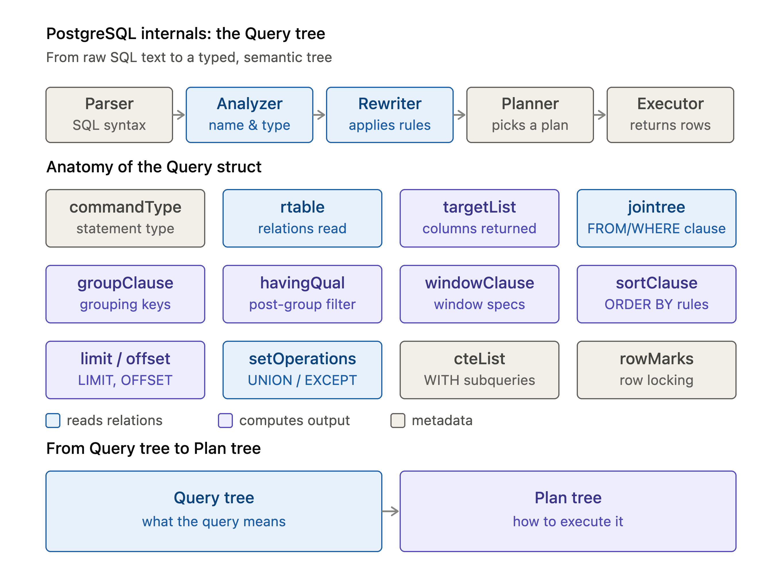
Last time in “Reading PostgreSQL”, we looked at how VACUUM acts as a clean-up crew for the debt created by INSERT, UPDATE, and DELETE operations.

Today, we turn our focus to query itself that is dissecting its internal anatomy to understand how PostgreSQL transforms a raw SQL string into a structured in-memory representation: the Query tree.

The Query Pipeline

Before diving into the Query struct and how PostgreSQL represents SQL internally, let’s recap the pipeline that a query traverses after reaching the backend.

As discussed in PostgreSQL Internals: Query Pipeline, query processing can be viewed as a five-stage assembly line, where the output of one stage becomes the input to the next:

1. Parser (gram.y)
   Performs syntactic analysis using the Flex lexer and Bison-generated parser. It verifies that the SQL conforms to PostgreSQL's grammar and produces a parse tree containing nodes such as RawStmt, SelectStmt, RangeVar, and ResTarget.

   At this stage, PostgreSQL understands the shape of the statement, but it does not yet resolve whether a referenced table or column actually exists.

2. Analyzer / Transformer
   Performs semantic analysis. It resolves names against PostgreSQL's system catalogs (pg_class, pg_attribute, pg_type, etc.), determines data types, establishes namespaces and scopes, resolves operators and functions, and converts the raw parse tree into an annotated Query tree.

3. Rewriter
   Applies PostgreSQL rewrite rules, including rules associated with views and other rewrite mechanisms. It can also add security-related qualifications where applicable.

   Importantly, the output of this stage is not necessarily one query. A single Query can be transformed into a list of Query trees.

4. Planner / Optimizer
   Takes the rewritten Query tree and determines how the query should execute. It considers possible access paths, join orders, join strategies, indexes, sorting, aggregation, and other execution alternatives using statistics and cost estimates.

   The result is a PlannedStmt containing a physical Plan tree.

5. Executor
   Executes the physical plan tree produced by the planner. It initializes the required executor nodes and recursively drives them to produce result tuples.

A simplified view is therefore:

SQL Statement → Parser (returns Parse Tree) → Analyzer (returns Query Tree) → Rewriter applies Rules, Views (returns a list of Query Tree) → Planner (return Plan Tree) → Executor → Result Rows

The important point for this article is the transition:

Raw SQL
   ↓
RawStmt / raw parse tree
   ↓
Query

The Query struct is where PostgreSQL has moved beyond simply understanding SQL syntax and has started building a semantic representation of what the query means.

The Query Struct

The Query node is defined in:

src/include/nodes/parsenodes.h

A simplified view of the structure looks like this:

typedef struct Query
{
    NodeTag         type;
    CmdType         commandType;
    QuerySource     querySource;
    uint64          queryId;
    bool            canSetTag;

    Node           *utilityStmt;

    int             resultRelation;

    bool            hasAggs;
    bool            hasWindowFuncs;
    bool            hasTargetSRFs;
    bool            hasSubLinks;
    bool            hasDistinctOn;
    bool            hasRecursive;
    bool            hasModifyingCTE;
    bool            hasForUpdate;
    bool            hasRowSecurity;
    bool            hasGroupRTE;
    bool            isReturn;

    List           *cteList;
    List           *rtable;
    List           *rteperminfos;

    FromExpr       *jointree;

    List           *mergeActionList;
    int             mergeTargetRelation;
    Node            *mergeJoinCondition;

    List           *targetList;

    OverridingKind  override;
    OnConflictExpr *onConflict;

    char           *returningOldAlias;
    char           *returningNewAlias;
    List           *returningList;

    List           *groupClause;
    bool            groupDistinct;
    List           *groupingSets;

    Node           *havingQual;

    List           *windowClause;
    List           *distinctClause;
    List           *sortClause;

    Node           *limitOffset;
    Node           *limitCount;
    LimitOption    limitOption;

    List           *rowMarks;

    Node           *setOperations;

    List           *constraintDeps;
    List           *withCheckOptions;

    ParseLoc        stmt_location;
    ParseLoc        stmt_len;
} Query;

Anatomy of the Query Struct

Once a statement passes through parsing and analysis, PostgreSQL has a much richer representation of it.

The parser primarily answers:

“Is this valid PostgreSQL syntax?”

The analyzer answers a much more interesting question:

“What does this statement actually refer to?”

For example, consider:

SELECT c.id
FROM companies c
WHERE c.revenue > 1000000;

After analysis, PostgreSQL needs to know:

• Which relation does companies refer to?

• What OID identifies that relation?

• Which attribute does c.id refer to?

• What data type does c.id have?

• What operator implements >?

• What type does 1000000 have in this expression?

• Which table does c refer to?

• Which expressions belong to the target list?

• Which expression represents the WHERE qualification?

The Query tree contains the information necessary for later stages to reason about those semantics.

1. Command Metadata

The first group of fields describes what kind of statement this is and which SQL features are present.

commandType

CmdType commandType;

commandType identifies the broad command represented by the Query:

CMD_SELECT
CMD_UPDATE
CMD_INSERT
CMD_DELETE
CMD_MERGE
CMD_UTILITY

For example:

SELECT * FROM companies;

will produce a Query whose commandType is:

CMD_SELECT

Whereas:

UPDATE companies
SET revenue = revenue * 1.1;

will have:

CMD_UPDATE

This gives later stages an immediate indication of the statement's nature.

querySource

QuerySource querySource;

This describes where the query came from.

A query may originate directly from the user, or it may have been generated as part of PostgreSQL's rewrite processing.

This distinction becomes particularly useful when PostgreSQL is dealing with rewritten queries.

queryId

uint64 queryId;

queryId represents a query identifier associated with the analyzed query.

It is important not to confuse this with the query ID displayed or used by pg_stat_statements as though Query.queryId itself were the statistics extension.

The query identifier is assigned as part of PostgreSQL's query-identification infrastructure and can be used by extensions such as pg_stat_statements to associate execution statistics with a normalized query identity.

The important distinction is:

Query.queryId
      │
      └── Query identification
              │
              └── Used by infrastructure/extensions
                  such as pg_stat_statements

It is not a transaction ID, object OID, or plan identifier.

2. Feature Flags

The Query node also contains several boolean fields:

bool hasAggs;
bool hasWindowFuncs;
bool hasTargetSRFs;
bool hasSubLinks;
bool hasDistinctOn;
bool hasRecursive;
bool hasModifyingCTE;
bool hasForUpdate;
bool hasRowSecurity;
bool hasGroupRTE;

These flags summarise important properties discovered during analysis.

For example:

SELECT department_id, count(*)
FROM employees
GROUP BY department_id;

contains an aggregate function.

Therefore:

hasAggs = true

Similarly:

SELECT name,
       row_number() OVER (ORDER BY salary)
FROM employees;

contains a window function, so:

hasWindowFuncs = true

These flags allow later processing stages to quickly determine whether particular query-processing features are involved without having to rediscover them from scratch.

3. Relations, Scope and the Range Table

One of the most important fields in Query is:

List *rtable;

This is the range table.

The range table contains RangeTblEntry structures representing the relations and other range-table items referenced by the query.

A simplified RangeTblEntry looks like:

typedef struct RangeTblEntry
{
    NodeTag type;
    RTEKind rtekind;

    Oid relid;

    Alias *alias;
    Alias *eref;

    Query *subquery;

    JoinType jointype;

    /* ... additional fields ... */
} RangeTblEntry;

The actual PostgreSQL structure contains considerably more information.

For a normal table reference:

SELECT *
FROM companies;

the corresponding RangeTblEntry contains information identifying the relation.

For example:

companies
    │
    ▼
RangeTblEntry
    │
    ├── rtekind = RTE_RELATION
    ├── relid   = <companies OID>
    └── ...

The important transformation is:

"companies"
     ↓
catalog lookup
     ↓
relation OID
     ↓
RangeTblEntry

This is one of the key differences between the raw parse tree and the analyzed Query tree.

4. Range Table Indexes

The range table is also important because other nodes refer to its entries by range-table index (rtindex).

For example:

typedef struct RangeTblRef
{
    NodeTag type;
    int rtindex;
} RangeTblRef;

If:

rtable[1] → companies
rtable[2] → employees

then a RangeTblRef with:

rtindex = 1

refers to the first range-table entry.

This gives PostgreSQL an internal relationship like:

Query
 │
 ├── rtable
 │    │
 │    ├── [1] → companies
 │    └── [2] → employees
 │
 └── jointree
      │
      ├── RangeTblRef(1)
      └── RangeTblRef(2)

The tree nodes don't need to repeatedly store the complete relation information. They can refer back to the appropriate RangeTblEntry.

5. TargetList: What Should the Query Produce?

Another critical field is:

List *targetList;

The target list represents the expressions that the query is interested in producing.

For:

SELECT c.id, c.name
FROM companies c;

the target list contains two TargetEntry nodes.

Conceptually:

targetList
   │
   ├── TargetEntry
   │      └── Var → c.id
   │
   └── TargetEntry
          └── Var → c.name

A simplified TargetEntry looks like:

typedef struct TargetEntry
{
    Expr       *expr;
    AttrNumber  resno;
    char       *resname;
    Index       ressortgroupref;
    bool        resjunk;
} TargetEntry;

6. The Var Node

The expr field can contain an expression node such as Var.

A simplified Var looks like:

typedef struct Var
{
    Expr        xpr;

    Index       varno;
    AttrNumber  varattno;
    Oid         vartype;

    /* ... additional properties ... */
} Var;

The important fields are:

varno

Identifies the range-table entry from which the value comes.

Conceptually:

varno = 1
     ↓
rtable[1]
     ↓
companies

varattno

Identifies the attribute within that relation.

For example:

varattno = 1

might correspond to the first user attribute of the relation.

vartype

Contains the PostgreSQL type OID.

For example:

23 → int4
25 → text

Therefore, an expression such as:

c.id

can eventually be represented conceptually as:

Var
 ├── varno    → companies
 ├── varattno → id
 └── vartype  → int4

This is a major semantic transformation.

The parser sees:

c.id

The analyzer turns that name into a structured reference to:

Range table entry
        +
attribute number
        +
data type

7. ResultRelation: Which Relation Is Being Modified?

For DML statements, PostgreSQL needs to identify the relation being modified.

This is represented by:

int resultRelation;

For example:

UPDATE companies
SET revenue = revenue * 1.1;

the resultRelation identifies the appropriate entry in the query's range table.

Conceptually:

rtable
 ├── [1] → companies
 │
 └── ...

resultRelation = 1

So:

resultRelation
      │
     ▼
rtable entry
      │
     ▼
companies

This allows later stages to determine which relation is the target of the modification.

8. CteList: Common Table Expressions

The Query also contains:

List *cteList;

This stores the query's Common Table Expressions (WITH clauses).

For example:

WITH high_value AS
(
    SELECT *
    FROM companies
    WHERE revenue > 1000000
)
SELECT *
FROM high_value;

The CTE is represented internally as a CommonTableExpr node in cteList.

Conceptually:

Query
 │
 ├── cteList
 │      │
 │      └── CommonTableExpr
 │              │
 │              └── Query
 │
 └── ...

A CTE therefore introduces another query representation nested inside the surrounding query structure.

9. JoinTree: FROM + WHERE Structure

One of the most interesting fields in Query is:

FromExpr *jointree;

The jointree represents the query's FROM/WHERE structure.

A simplified FromExpr is:

typedef struct FromExpr
{
    NodeTag type;

    List *fromlist;

    Node *quals;
} FromExpr;

It contains two important pieces:

fromlist

The relations and joins appearing in the FROM clause.

quals

The qualification expression, which generally corresponds to the WHERE condition.

For example:

SELECT *
FROM companies
WHERE revenue > 1000000;

can be visualized as:

FromExpr
 │
 ├── fromlist
 │      │
 │      └── RangeTblRef
 │              │
 │              └── companies
 │
 └── quals
        │
        └── 
            ├── Var → companies.revenue
            └── Const → 1000000

Notice that the WHERE expression is not represented as a separate "WHERE node."

It is stored as the quals expression tree.

10. Representing JOINs

For a query such as:

SELECT *
FROM companies c
JOIN employees e
    ON c.id = e.company_id;

the FROM structure contains a JoinExpr.

A simplified representation is:

typedef struct JoinExpr
{
    JoinType jointype;

    Node *larg;
    Node *rarg;

    List *usingClause;

    Node *quals;

    Alias *join_using_alias;
    int rtindex;
} JoinExpr;

Conceptually:

JoinExpr
 │
 ├── jointype = JOIN_INNER
 │
 ├── larg
 │     └── RangeTblRef → companies
 │
 ├── rarg
 │     └── RangeTblRef → employees
 │
 └── quals
       └── =
           ├── Var → companies.id
           └── Var → employees.company_id

So the query's relational structure can be represented as a tree:

                 JoinExpr
                /        \
               /          \
       companies        employees
              \            /
               \          /
                join condition

This representation gives later stages a structured description of the query's relational topology.

11. GroupClause and Aggregation

Consider:

SELECT company_id, count(*)
FROM employees
GROUP BY company_id;

The Query contains:

List *groupClause;

which represents the grouping specification.

The aggregate itself contributes to the expression tree in the target list.

Conceptually:

Query
 │
 ├── targetList
 │      ├── Var → company_id
 │      └── Aggref
 │             └── count(*)
 │
 └── groupClause
        └── company_id

This separation is useful because PostgreSQL needs to reason independently about:

• what values are produced,

• what expressions are aggregated,

• and what expressions define the grouping.

12. HavingQual

HAVING is different from WHERE.

Consider:

SELECT company_id, count(*)
FROM employees
GROUP BY company_id
HAVING count(*) > 10;

The HAVING condition is represented by:

Node *havingQual;

Conceptually:

GROUP BY
    ↓
Aggregation
    ↓
HAVING
    ↓
Result

Whereas a WHERE condition generally belongs to:

jointree->quals

This distinction is important because the two predicates operate at different logical stages.

13. Window Functions

Window specifications are represented using:

List *windowClause;

For example:

SELECT
    name,
    salary,
    row_number() OVER (ORDER BY salary DESC)
FROM employees;

The query contains information describing the window specification:

windowClause
    │
    └── Window specification
            │
            └── ORDER BY salary DESC

The window function itself appears in the relevant expression tree.

14. SortClause

ORDER BY information is represented through:

List *sortClause;

For:

SELECT *
FROM employees
ORDER BY salary DESC;

the query representation records the expression being sorted and the associated sort semantics.

Conceptually:

sortClause
    │
    └── salary
          │
          └── DESC

The important distinction is that the Query describes what ordering is required.

It is the planner that later decides how to achieve that ordering.

For example, the planner might determine that an index can provide the required ordering, or that an explicit sort operation is necessary.

15. LimitOffset and LimitCount

LIMIT and OFFSET are represented using:

Node *limitOffset;
Node *limitCount;
LimitOption limitOption;

For:

SELECT *
FROM employees
LIMIT 10
OFFSET 20;

the query representation contains expressions corresponding to:

limitOffset → 20
limitCount  → 10

Again, the Query describes the semantic requirement.

The planner and executor determine how that requirement is physically implemented.

16. SetOperation

PostgreSQL also needs to represent set operations such as:

SELECT id FROM companies
UNION
SELECT id FROM employees;

The relevant information is stored through:

Node *setOperations;

This can represent operations such as:

UNION
INTERSECT
EXCEPT

and their associated query structures.

Conceptually:

SetOperation
      │
      ├── left query
      │
      └── right query

17. RowMarks

Queries involving row-level locking, such as:

SELECT *
FROM employees
FOR UPDATE;

carry locking information through:

List *rowMarks;

This allows PostgreSQL to preserve the semantic requirement that selected rows must be locked.

The planner later translates this requirement into an appropriate execution strategy.

18. rteperminfos: Separating Permissions from Range Table Entries

Alongside rtable, the Query struct also carries:

List *rteperminfos;

This list holds RTEPermissionInfo structures, one per relation that actually needs an access-control check – which is a smaller set than rtable itself, since not every range table entry represents a checkable relation (a subquery RTE or join RTE doesn't need its own permission check, for instance).

A simplified RTEPermissionInfo looks like:

typedef struct RTEPermissionInfo
{
    NodeTag     type;

    Oid         relid;
    bool        inh;

    AclMode     requiredPerms;
    Oid         checkAsUser;

    Bitmapset  *selectedCols;
    Bitmapset  *insertedCols;
    Bitmapset  *updatedCols;
} RTEPermissionInfo;

Each RangeTblEntry that needs checking stores an index (perminfoindex) back into rteperminfos, rather than embedding the permission fields directly on itself:

rtable
 ├── [1] companies  ──── perminfoindex ────┐
 └── [2] employees  ──── perminfoindex ──┐ │
                                          ▼ ▼
                                   rteperminfos
                                    ├── [1] companies: requiredPerms, selectedCols...
                                    └── [2] employees: requiredPerms, selectedCols...

Why split it out at all? Because permission checking and range-table membership are logically different concerns. A view expands into multiple RTEs during rewriting, but the permission check should still apply to the view as the user wrote it, not to each underlying table separately. Keeping RTEPermissionInfo as its own list lets PostgreSQL track who needs to be allowed to do what independently of which relations the plan will actually touch – the two lists can diverge as the query tree is rewritten and expanded, without one bloating or corrupting the other.

19. Tracking the Original SQL Location

Finally, the Query structure contains:

ParseLoc stmt_location;
ParseLoc stmt_len;

These fields record the location and length of the statement within the original query text.

This is useful because PostgreSQL does not need to duplicate the complete SQL text inside every parse-tree node merely to remember where something originated.

Instead, nodes can retain source-location information that points back into the original query string.

Conceptually:

Original query buffer

SELECT c.id, count(*)
FROM companies c
...

^
|
stmt_location

<-------- stmt_len -------->

This source-location information is also useful for producing accurate error messages and other diagnostics.

Putting Everything Together

Let's take a concrete example:

SELECT c.id, count(*)
FROM companies c
JOIN employees e
    ON c.id = e.company_id
GROUP BY c.id;

At the SQL level, we can think about the query as:

SELECT
    c.id,
    count(*)

FROM
    companies c
    JOIN employees e
        ON c.id = e.company_id

GROUP BY
    c.id

After analysis, PostgreSQL has enough information to construct a semantic representation roughly like:

Query
│
├── commandType
│     └── CMD_SELECT
│
├── rtable
│     ├── [1] → companies
│     └── [2] → employees
│
├── targetList
│     ├── TargetEntry
│     │      └── Var
│     │           ├── varno → 1
│     │           ├── varattno → id
│     │           └── vartype → int4
│     │
│     └── TargetEntry
│            └── Aggref
│                 └── count(*)
│
├── jointree
│     └── FromExpr
│           │
│           └── JoinExpr
│               ├── larg → RangeTblRef(1)
│               ├── rarg → RangeTblRef(2)
│               └── quals
│                     └── c.id = e.company_id
│
└── groupClause
      └── c.id

This is the important conceptual leap:

SQL text

c.id

becomes something closer to:

Var
 ├── varno
 ├── varattno
 └── vartype

And:

SQL relation

companies

becomes:

RangeTblEntry
 └── relid → relation OID

And:

SQL JOIN

companies c
JOIN employees e
ON c.id = e.company_id

becomes a structured tree:

JoinExpr
├── left relation
├── right relation
└── join qualification

PostgreSQL has therefore transformed human-readable SQL names into a graph/tree of strongly typed internal nodes.

Conclusion

A Query is PostgreSQL's answer to what does this SQL actually mean – names resolved to Vars and RangeTblEntrys, structure captured in jointree, intent captured in fields like groupClause, sortClause, and rteperminfos. It describes the query fully, but not how to run it – that's the planner's job, and where we'll head next.